Working with Piecewise Continuous Functions: IntervalData

Introduction

The IntervalData class is a subclass of IntervalDict class of Portion, used to hold and work with data (or function) that is piecewise continuous. The most obvious usecase is spectral data, where a continuous spectrum (for example from the Sun) can be then filtered in two distinct bands. The filters can be box filters (1.0 at the pass band, zero otherwise) or more complex filters with tapered edges.

When combined with interpolators and resampling, this provides a very powerful framework to simulate light (or generally radiofrequency) spectrum, interacting with filters or other surfaces that modify the amplitude and spectral properties as it goes through them or bounces off them.

We have to start with the opticks package import as well as some other useful packages.

# If opticks import fails, try to locate the module
# This can happen building the docs
import os

try:
    import importlib.util

    if importlib.util.find_spec("opticks") is None:
        raise ModuleNotFoundError
except ModuleNotFoundError:
    os.chdir(os.path.join("..", "..", ".."))
    os.getcwd()

import numpy as np
from astropy.visualization import quantity_support

from opticks import P, u

# astropy units support for matplotlib
quantity_support()

%matplotlib inline


import warnings

warnings.filterwarnings("always")

Initialising IntervalData

As a simple example, we start with a filter defined from -10 Hz to +10 Hz. It is transparent between -4 Hz and 0 Hz and between 2 Hz and 5 Hz. Outside the range of validity, the filter is undefined and returns None, inside the range of validity it returns zero where it is “non-transparent” and 1.0 where it is “transparent”.

Also, there is no such thing as a negative frequency in the absolute sense, but it is possible in the relative sense. It matters little for this example, though may be worth mentioning for the sake of clarity.

from opticks.utils.interval_data import IntervalData

data = P.IntervalDict()
# interval of validity
validity = P.closed(-10 * u.Hz, 10 * u.Hz)
data[validity] = 0
# data proper
first_rng = P.closed(-4 * u.Hz, 0 * u.Hz)
data[first_rng] = 1.0
second_rng = P.closed(2 * u.Hz, 5 * u.Hz)
data[second_rng] = 1.0

filter = IntervalData(data)

# filter definition
print(filter)
# interval of validity
print(filter.domain())

# data inside interval of validity but zero
print(filter.get_value((8 * u.Hz)))
# data outside interval of validity: None
print(filter.get_value((12 * u.Hz)))

{[<Quantity -10. Hz>,<Quantity -4. Hz>) | (<Quantity 0. Hz>,<Quantity 2. Hz>) | (<Quantity 5. Hz>,<Quantity 10. Hz>]: 0, [<Quantity -4. Hz>,<Quantity 0. Hz>] | [<Quantity 2. Hz>,<Quantity 5. Hz>]: 1.0}
[<Quantity -10. Hz>,<Quantity 10. Hz>]
0.0
None

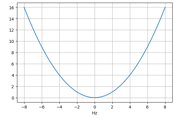
For something a bit more interesting, we will define a quadratic function, though we will take discrete steps and initialise an interpolator, rather than using the analytical function directly.

The data is defined from -8 to + 8 Hz, therefore shorter than the filter definition. This will be important later, when we apply the “filter” to this function.

from opticks.utils.math_utils import InterpolatorWithUnits, InterpolatorWithUnitTypes

target_range = P.closed(-8 * u.Hz, 8 * u.Hz)

x = np.linspace(target_range.lower, target_range.upper, num=100, endpoint=True)

y = (0.5 * x.value) ** 2

ipol = InterpolatorWithUnits.from_ipol_method(
    InterpolatorWithUnitTypes.AKIMA, x, y, extrapolate=True
)

main_funct = IntervalData.from_interpolator(ipol)

print(main_funct)

{[<Quantity -8. Hz>,<Quantity 8. Hz>]: <opticks.utils.math_utils.InterpolatorWithUnits object at 0x7f4e4b208e10>}

Plotting the Data

The IntervalDict objects can be plotted easily. It is a matplotlib based convenience class for rapid visualisation and does not enable extensive customisation via the interface.

from opticks.utils.interval_data import IntervalDataPlot

interval_data_dict = {"data": main_funct, "filter": filter}

plot = IntervalDataPlot(interval_data_dict)

While the out-of-the-box formatting is sensible, it is possible to change things once the plot is populated. The fig and ax objects are also available for further customisation.

plot2 = IntervalDataPlot({"data": main_funct, "filter": filter})

# customisation via the limited convenience method
plot2.set_plot_style(
    xlabel="x axis title (Hz)",
    ylabel="user defined y axis title",
    height=10 * u.cm,
    width=15 * u.cm,
)

# customisation via the ax object
# example only, can be also done via set_plot_style
plot2.ax.set_title("Filter and Data")

Text(0.5, 1.0, 'Filter and Data')

It is also possible for the IntervalData objects to plot themselves for even easier data visualisation.

main_funct.plot()

<opticks.utils.interval_data.IntervalDataPlot at 0x7f4e4b285f10>

Combining IntervalData Objects

The next step is to combine the filter and the main function. This combine operation is defined as “stacking” the mathematical functions, interpolators or constants together in a list, for the proper internal regions of validity. Therefore, no resampling or evaluation actually takes place. The interpolators do not need to interpolate or extrapolate. The underlying IntervalDict implementation takes care of the interval arithmetic and knows the intersections.

Also, the region of validity for the combined IntervalDict is necessarily the intersection of the two, as the behaviour of filter or main_funct is not defined outside their respective regions of validity. The combined item still has the larger interval of validity, but these ranges yield None as the value. This behaviour can be changed with the missing key for the combine operation, but should be done cautiously.

To get the “stack” of functions at a certain point or region is possible using the get function. In this example, we have the interpolator and the value of 1.0.

from opticks.utils.interval_data import FunctCombinationMethod

filter.combination_method = FunctCombinationMethod.MULTIPLY
filtered_main = main_funct.combine(filter)

print(filtered_main)

# sample point x
x = 3 * u.Hz

# stack of functions at x
print(filtered_main.get(x))

{[<Quantity -10. Hz>,<Quantity -8. Hz>) | (<Quantity 8. Hz>,<Quantity 10. Hz>]: None, [<Quantity -8. Hz>,<Quantity -4. Hz>) | (<Quantity 0. Hz>,<Quantity 2. Hz>) | (<Quantity 5. Hz>,<Quantity 8. Hz>]: [<opticks.utils.math_utils.InterpolatorWithUnits object at 0x7f4e4b208e10>, 0], [<Quantity -4. Hz>,<Quantity 0. Hz>] | [<Quantity 2. Hz>,<Quantity 5. Hz>]: [<opticks.utils.math_utils.InterpolatorWithUnits object at 0x7f4e4b208e10>, 1.0]}
[<opticks.utils.math_utils.InterpolatorWithUnits object at 0x7f4e4b208e10>, 1.0]

In the example above, the combination method of the filter is set to MULTIPLY, before combining the two objects. The combine method does not define how the two IntervalData should be combined arithmetically. Therefore, when two IntervalData objects are combined and we would like to evaluate the data at a specific point, we have to define whether a multiplication or a summation operation is to be used.

When an IntervalData object is created, the default combination method is UNDEFINED. A combination is only possible between objects of compatible types. Objects of SUM types can be combined only with other objects of SUM or UNDEFINED types, where summation becomes the method for the entire combination sequence. The same logic goes for MULTIPLY, which can be combined only with MULTIPLY or UNDEFINED type objects.

Note that, a SUM object cannot be combined with a MULTIPLY type object, as both might have various functions stacked and need to be evaluated with its own combination method. To combine such IntervalData objects, one of them should be resampled (see below), making it UNDEFINED again. After resampling, they can be combined normally.

Similarly, an UNDEFINED object cannot be directly combined with another UNDEFINED object. One of them should be set to SUM or MULTIPLY, so that the combined object knows how to handle the combination.

# the combination type for the main function is by default undefined
print(main_funct.combination_method)

# the combination type for the combined filter is set to multiplication
print(filtered_main.combination_method)

FunctCombinationMethod.UNDEFINED
FunctCombinationMethod.MULTIPLY

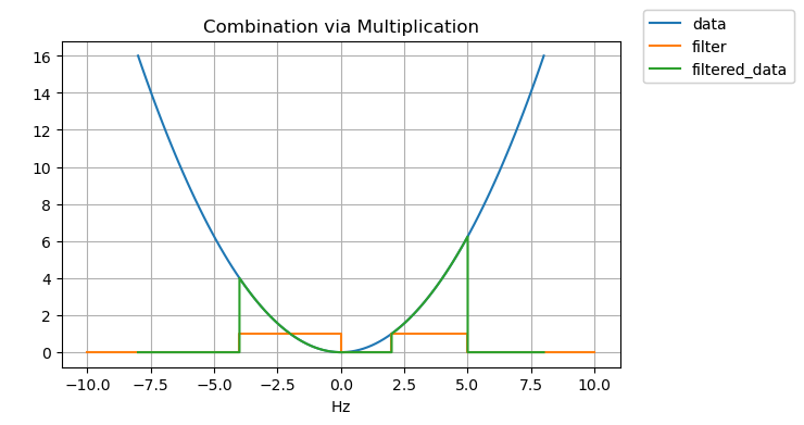
Now that we defined how to combine the two IntervalData objects (in this case via multiplication), the get_value function evaluates all the “stacked” functions at the requested point and yields the result.

# value at x (multiply all values at x)
print(filtered_main.get_value(x))

# stack of functions within the target range
target_range = P.closed(1 * u.Hz, 4 * u.Hz)
print(filtered_main.get(target_range))

2.2499999999999996
{[<Quantity 1. Hz>,<Quantity 2. Hz>): [<opticks.utils.math_utils.InterpolatorWithUnits object at 0x7f4e4b208e10>, 0], [<Quantity 2. Hz>,<Quantity 4. Hz>]: [<opticks.utils.math_utils.InterpolatorWithUnits object at 0x7f4e4b208e10>, 1.0]}

We can plot the resulting piecewise continuous function to see the effect of “filtering”, or combining the two functions with a multiplication operation.

interval_data_dict = {
    "data": main_funct,
    "filter": filter,
    "filtered_data": filtered_main,
}

plot = IntervalDataPlot(interval_data_dict)

plot.set_plot_style(title="Combination via Multiplication")

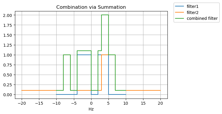
To illustrate how summation works, we will define another “filter” and combine with the first, explicitly defining a summation type combination. Then we can query any point on the list.

data = P.IntervalDict()
# interval of validity
validity = P.closed(-20 * u.Hz, 20 * u.Hz)
data[validity] = 0.1
# data proper
first_rng = P.closed(-8 * u.Hz, -6 * u.Hz)
data[first_rng] = 1.0
second_rng = P.closed(3 * u.Hz, 7 * u.Hz)
data[second_rng] = 1.0

# filter2 definition
filter2 = IntervalData(data)

# filter 2 output
print(filter2)

# combine the two filters
filter.combination_method = FunctCombinationMethod.SUM
combined_filter = filter2.combine(filter)


# combined filter output
print(combined_filter)

# value at x (sum all values at x)
x = 4.5 * u.Hz

print(combined_filter.get_value(x))

{[<Quantity -20. Hz>,<Quantity -8. Hz>) | (<Quantity -6. Hz>,<Quantity 3. Hz>) | (<Quantity 7. Hz>,<Quantity 20. Hz>]: 0.1, [<Quantity -8. Hz>,<Quantity -6. Hz>] | [<Quantity 3. Hz>,<Quantity 7. Hz>]: 1.0}
{[<Quantity -20. Hz>,<Quantity -10. Hz>) | (<Quantity 10. Hz>,<Quantity 20. Hz>]: None, [<Quantity -10. Hz>,<Quantity -8. Hz>) | (<Quantity -6. Hz>,<Quantity -4. Hz>) | (<Quantity 0. Hz>,<Quantity 2. Hz>) | (<Quantity 7. Hz>,<Quantity 10. Hz>]: [0.1, 0], [<Quantity -8. Hz>,<Quantity -6. Hz>] | (<Quantity 5. Hz>,<Quantity 7. Hz>]: [1.0, 0], [<Quantity -4. Hz>,<Quantity 0. Hz>] | [<Quantity 2. Hz>,<Quantity 3. Hz>): [0.1, 1.0], [<Quantity 3. Hz>,<Quantity 5. Hz>]: [1.0, 1.0]}
2.0

It is useful to plot all three filters to visualise the end result.

interval_data_dict = {
    "filter1": filter,
    "filter2": filter2,
    "combined filter": combined_filter,
}

plot = IntervalDataPlot(interval_data_dict)

plot.set_plot_style(title="Combination via Summation")

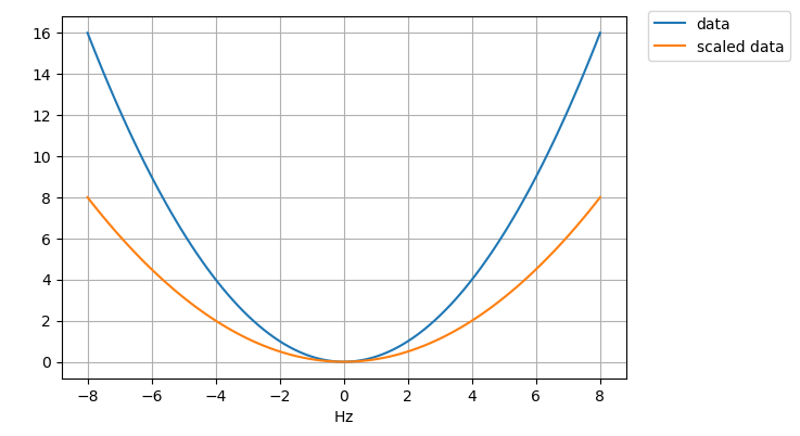
It is possible to scale the IntervalData objects with a scalar. This is achieved via a combine operation under the hood. We can plot the main function and a 1/2 scaling to see the end result.

scaled_main = main_funct.scale(0.5)

interval_data_dict = {"data": main_funct, "scaled data": scaled_main}

plot = IntervalDataPlot(interval_data_dict)

Flattening the Functions Stack: Resampling

After successive combine operations, the functions stack can pile high, with multiple interpolations slowing down the operations. The resample function ‘flattens’ the stack, via a resampling and setting up a new interpolator.

The resampling is done for each atomic interval within the IntervalData object. This process decomposes all the intervals into atomic intervals, processes them and puts them back together into a new IntervalData object

The following example shows the atomic intervals.

# interval: funct view of the IntervalDict
atomic_int = filtered_main.as_atomic()

# List atomic intervals and corresponding functions
for interval, functs in atomic_int:
    print(interval, functs)

[<Quantity -10. Hz>,<Quantity -8. Hz>) None
(<Quantity 8. Hz>,<Quantity 10. Hz>] None
[<Quantity -8. Hz>,<Quantity -4. Hz>) [<opticks.utils.math_utils.InterpolatorWithUnits object at 0x7f4e4b208e10>, 0]
(<Quantity 0. Hz>,<Quantity 2. Hz>) [<opticks.utils.math_utils.InterpolatorWithUnits object at 0x7f4e4b208e10>, 0]
(<Quantity 5. Hz>,<Quantity 8. Hz>] [<opticks.utils.math_utils.InterpolatorWithUnits object at 0x7f4e4b208e10>, 0]
[<Quantity -4. Hz>,<Quantity 0. Hz>] [<opticks.utils.math_utils.InterpolatorWithUnits object at 0x7f4e4b208e10>, 1.0]
[<Quantity 2. Hz>,<Quantity 5. Hz>] [<opticks.utils.math_utils.InterpolatorWithUnits object at 0x7f4e4b208e10>, 1.0]

The resampling is carried out respecting the content of the functions stack at each atomic interval. Assuming a MULTIPLY type stack:

• If one item of the functions stack is None, then the entire interval value is set to None

• If one item of the functions stack is zero, then the entire interval value is set to zero.

• If all the items of the functions stack are numbers, then the entire interval value is set to the multiplication of these numbers.

• Finally, if one item of the multiple item functions stack is a continuous function or interpolator, then the entire interval value is resampled.

In this example, the resampling for the first two intervals in the list would automatically result in None, the next three intervals automatically zero and the last two intervals would be resampled.

A SUM type stack would be handled similarly, with summation of the stacked values instead of multiplication.

The sample sizes are important only when an interpolation is needed. The sample_size argument instructs the method to set the sample size accordingly for each atomic interval where interpolation is needed. The samples are computed by dividing the interval by the stepsize and rounding down to convert them into integers.

filtered_main.sample_size = 150

resampled_filt_main = filtered_main.resample()

# original
print(filtered_main)

# resampled
print(resampled_filt_main)

{[<Quantity -10. Hz>,<Quantity -8. Hz>) | (<Quantity 8. Hz>,<Quantity 10. Hz>]: None, [<Quantity -8. Hz>,<Quantity -4. Hz>) | (<Quantity 0. Hz>,<Quantity 2. Hz>) | (<Quantity 5. Hz>,<Quantity 8. Hz>]: [<opticks.utils.math_utils.InterpolatorWithUnits object at 0x7f4e4b208e10>, 0], [<Quantity -4. Hz>,<Quantity 0. Hz>] | [<Quantity 2. Hz>,<Quantity 5. Hz>]: [<opticks.utils.math_utils.InterpolatorWithUnits object at 0x7f4e4b208e10>, 1.0]}
{[<Quantity -10. Hz>,<Quantity -8. Hz>) | (<Quantity 8. Hz>,<Quantity 10. Hz>]: None, [<Quantity -8. Hz>,<Quantity -4. Hz>): <opticks.utils.math_utils.InterpolatorWithUnits object at 0x7f4e4ab9b700>, [<Quantity -4. Hz>,<Quantity 0. Hz>]: <opticks.utils.math_utils.InterpolatorWithUnits object at 0x7f4e4ab9b750>, (<Quantity 0. Hz>,<Quantity 2. Hz>): <opticks.utils.math_utils.InterpolatorWithUnits object at 0x7f4e4ab9be30>, [<Quantity 2. Hz>,<Quantity 5. Hz>]: <opticks.utils.math_utils.InterpolatorWithUnits object at 0x7f4e4ab9bed0>, (<Quantity 5. Hz>,<Quantity 8. Hz>]: <opticks.utils.math_utils.InterpolatorWithUnits object at 0x7f4e4ab9bcf0>}

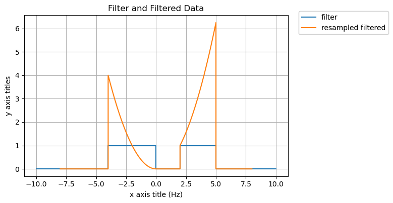
Inspecting the output, we can see that the intervals with None and zero are still merged as a single, non-atomic interval, whereas the interpolated interval is now made up of two non-adjacent parts.

We can plot all three functions to inspect the results visually.

plot2 = IntervalDataPlot({"filter": filter, "resampled filtered": resampled_filt_main})
plot2.set_plot_style(
    xlabel="x axis title (Hz)",
    ylabel="y axis titles",
    height=10 * u.cm,
    width=15 * u.cm,
)

# example only, can be also done via set_plot_style
plot2.ax.set_title("Filter and Filtered Data")

Text(0.5, 1.0, 'Filter and Filtered Data')

Mathematical Operations on the IntervalData Objects

Some mathematical operations can be carried out on the IntervalData objects. For example, they can be integrated within a certain range.

### Integral over a domain

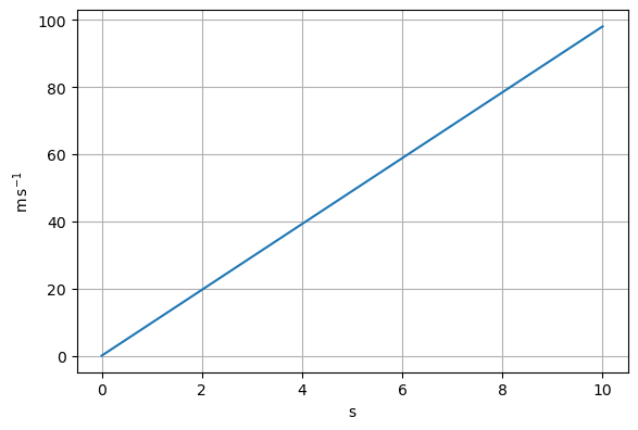
Let’s define a simple example with the velocity of a free falling object.

from astropy.units import Unit

duration = P.closed(0 * u.s, 10 * u.s)

t = np.linspace(duration.lower, duration.upper, num=100, endpoint=True)

v = 9.81 * Unit("m/s^2") * t

ipol = InterpolatorWithUnits.from_ipol_method(
    InterpolatorWithUnitTypes.AKIMA, t, v, extrapolate=True
)

free_fall_funct = IntervalData.from_interpolator(ipol)

free_fall_funct.plot()

<opticks.utils.interval_data.IntervalDataPlot at 0x7f4eca137290>

The time integral of the velocity is the position, or in this case, the distance travelled. The true value is simply \(1/2 \times gt^2\).

integral = free_fall_funct.integrate()

print(f"True value: {0.5 * 9.81 * Unit('m/s^2') * t[-1] ** 2}")
print(f"Computed value: {integral}")

True value: 490.5 m
Computed value: 490.50000000000006 m

It is also possible to query a limited duration.

limited_rng = P.closed(4 * u.s, 6 * u.s)
integral = free_fall_funct.integrate(limited_rng)

print(f"Computed value: {integral}")
print(
    f"True value: {0.5 * 9.81 * Unit('m/s^2') * (limited_rng.upper**2 - limited_rng.lower**2)}"
)

Computed value: 98.10000000000001 m
True value: 98.10000000000001 m

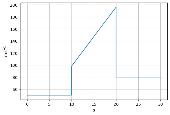
We can make this example more complicated and see whether it works.

data = P.IntervalDict()

# segment 1
duration_1 = P.closed(0 * u.s, 10 * u.s)
vel_1 = 50.0 * u.m / u.s
data[duration_1] = vel_1

# segment 2
duration_2 = P.closed(10 * u.s, 20 * u.s)
t = np.linspace(duration_2.lower, duration_2.upper, num=100, endpoint=True)
v = 9.81 * Unit("m/s^2") * t

ipol = InterpolatorWithUnits.from_ipol_method(
    InterpolatorWithUnitTypes.AKIMA, t, v, extrapolate=True
)

data[duration_2] = ipol

# segment 3
duration_3 = P.closed(20 * u.s, 30 * u.s)
vel_3 = 80.0 * u.m / u.s
data[duration_3] = vel_3

free_fall_funct = IntervalData(data)

free_fall_funct.plot()

<opticks.utils.interval_data.IntervalDataPlot at 0x7f4e4aa298e0>

integral = free_fall_funct.integrate()

true_integ = (
    vel_1 * (duration_1.upper - duration_1.lower)
    + 0.5 * 9.81 * Unit("m/s^2") * (duration_2.upper**2 - duration_2.lower**2)
    + vel_3 * (duration_3.upper - duration_3.lower)
)

print(f"True value: {true_integ}")
print(f"Computed value: {integral}")

True value: 2771.5 m
Computed value: 2771.5 m