Interpolation with Units

The interpolation algorithms within opticks use piecewise polynomials to interpolate discrete data. The underlying library is of course scipy, which offers Cubic Spline based as well as monotone interpolators. The latter prevents overshoot but may be less accurate locally, particularly for smooth data.

Unlike numpy, the units library astropy.units does not directly support scipy. Therefore the unit support for the interpolators had to be defined from scratch.

For this, PPolyWithUnits and InterpolatorWithUnits are developed, mimicking the relationship between scipy class .PPoly and interpolators like CubicHermiteSpline.

We have to start with the opticks package import as well as some other useful packages.

# If opticks import fails, try to locate the module
# This can happen building the docs
import os

try:
    import importlib.util

    if importlib.util.find_spec("opticks") is None:
        raise ModuleNotFoundError
except ModuleNotFoundError:
    os.chdir(os.path.join("..", "..", ".."))
    os.getcwd()

import numpy as np
from astropy.visualization import quantity_support

from opticks import u

# astropy units support for matplotlib
quantity_support()

%matplotlib inline

import warnings

from matplotlib import pyplot as plt

warnings.filterwarnings("always")

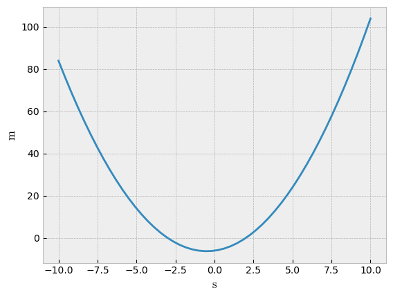
First we can check whether the scipy interpolators really ignore units with a simple example. We will create a quadratic polynomial with the units of time and distance.

\[y(t) = (t-2)(t+3) = t^2 + t- 6\]

This form shows the roots clearly, which will be useful later. The interpolator is set up from discrete points between -10 sec and +10 sec.

The derivative is simply:

\[\dot{y}(t) = 2t + 1\]

And the integral is:

\[\int y dt = \frac{t^3}{3} + \frac{t^2}{2}- 6t + C\]

from scipy.interpolate import Akima1DInterpolator

# define the polynomial with discrete samples
t = np.linspace(-10, 10, endpoint=True) * u.s
y = (t.value - 2) * (t.value + 3) * u.m

# set plot style
plt.style.use("bmh")

# plot the data for easy visualisation
plt.plot(t, y)

[<matplotlib.lines.Line2D at 0x72a10eda05c0>]

# prepare interpolator (causes UnitStrippedWarning)
ipl_no_units = Akima1DInterpolator(t, y, method="akima")

# interpolation target value
t_tgt = 4.1 * u.s

# result should be in m
print(ipl_no_units(t_tgt))

# same input time in minutes - the result should have been the same
print(ipl_no_units(t_tgt.to(u.min)))

14.909999999999997
-5.926997222222222

Two observations can be made: While the inputs have units, the result of the interpolation has no units, which resulted in a difference when the same time is expressed in minutes. And we received a UnitStrippedWarning that explains why; there is a downcasting within the interpolation that deletes the units.

On the other hand, the numpy linear interpolation works out of the box.

print(np.interp(t_tgt, t, y))

14.951311953352768 m

Now try the new InterpolatorWithUnits.

from opticks.utils.math_utils import InterpolatorWithUnits, InterpolatorWithUnitTypes

# choose the interpolator type
ipol_type = InterpolatorWithUnitTypes.AKIMA

# init the interpolator
ipol = InterpolatorWithUnits.from_ipol_method(ipol_type, t, y, extrapolate=True)

# result should be in m
print(ipol(t_tgt))

# same input time in minutes - the result should be the same
print(ipol(t_tgt.to(u.min)))

# exact value
print((t_tgt.value - 2) * (t_tgt.value + 3) * u.m)

14.909999999999997 m
14.909999999999997 m
14.909999999999997 m

The initialisation is the same as the standard Akima1DInterpolator, accepting all the args and kwargs necessary, with the exception of method keyword for Akima - the InterpolatorWithUnitTypes.MAKIMA takes care of this by initialising a Modified Akima scheme.

The other thing to note is that the unit conversions are handled automatically. It does not matter whether the input is given in seconds or minutes, the result is the same in both cases.

However, the unit checks are strict. For example, if the unit of the interpolation target t_tgt does not match the unit of the t values, an exception will be thrown. Similarly, a float would not be accepted in this case, as there is no way to know how to interpret a float - is it in seconds or hours?

Other functions from the scipy interpolators are also implemented.

deriv = ipol.derivative(1)
print(f"Derivative: {deriv(t_tgt)}")
print(f"Derivative: {(2 * t_tgt.value + 1) * u.m / u.s} (exact value)")


antideriv = ipol.antiderivative(1)
print(f"Antiderivative: {antideriv(t_tgt):.6}")
# this is essentially the definite integral from t_begin to t_tgt
t_begin = t[0]
int_begin = (
    ((t_begin.value**3 / 3) + (t_begin.value**2 / 2) - 6 * t_begin.value) * u.m * u.s
)
int_tgt = ((t_tgt.value**3 / 3) + (t_tgt.value**2 / 2) - 6 * t_tgt.value) * u.m * u.s
print(f"Antiderivative: {int_tgt - int_begin:.6} (exact value)")


a = -1 * u.s
b = 4.1 * u.s
print(f"Definite Integral from {a} to {b}: {ipol.integrate(a, b):.6}")
int_begin = ((a.value**3 / 3) + (a.value**2 / 2) - 6 * a.value) * u.m * u.s
int_tgt = ((b.value**3 / 3) + (b.value**2 / 2) - 6 * b.value) * u.m * u.s
print(f"Definite Integral from {a} to {b}: {int_tgt - int_begin} (exact value)")

print("--------")

solve_tgt = 20 * u.m
print(f"Solve at {solve_tgt}: {ipol.solve(solve_tgt)}")

print(f"Roots : {ipol.roots()}")

Derivative: 9.2 m / s
Derivative: 9.2 m / s (exact value)
Antiderivative: 230.112 m s
Antiderivative: 230.112 m s (exact value)
Definite Integral from -1.0 s to 4.1 s: 0.612 m s
Definite Integral from -1.0 s to 4.1 s: 0.6119999999999957 m s (exact value)
--------
Solve at 20.0 m: [-5.62347538  4.62347538] s
Roots : [-3.  2.] s

Also note that the antiderivative is from the beginning of the x axis data (in this case -10 seconds) until the requested point (in this case t_tgt). integrate is similar, but the beginning and end points are explicitly defined.

The other way to initialise the InterpolatorWithUnits is to ingest an external interpolator and add units. That said, units are not strictly required.

We can show both in an example.

# Init scipy interpolator, strip units
scipy_ipol = Akima1DInterpolator(t.value, y.value, method="makima")

# Init the Interpolator with units, but delete the units of y
ipol2 = InterpolatorWithUnits(scipy_ipol, t.unit, None)

# result should be without dimensions
print(ipol2(t_tgt))

14.910166202386884

Finally, let’s see how another interpolator can be initialised with args and kwargs passed on properly.

# Array containing derivatives of the dependent variable.
# Set with zeros, probably not realistic, but ok for this example
dydx = np.zeros_like(t)

ipol3 = InterpolatorWithUnits.from_ipol_method(
    InterpolatorWithUnitTypes.CUBICHERMITESPL, t, y, dydx=dydx
)
print(ipol3(t_tgt), InterpolatorWithUnitTypes.CUBICHERMITESPL.name)


ipol4 = InterpolatorWithUnits.from_ipol_method(
    InterpolatorWithUnitTypes.CUBICSPL, t, y, bc_type="not-a-knot"
)

print(ipol4(t_tgt), InterpolatorWithUnitTypes.CUBICSPL.name)

15.034782755102038 m CUBICHERMITESPL
14.909999999999997 m CUBICSPL