Defining an Aperture

Introduction

In this tutorial we will define apertures, starting from a simple one and increasing the complexity.

The aperture can be a simple circular one, or with an obscuration and even with spiders to hold the secondary mirror in place. The Amplitude (through the aperture) simply describes how much light is let in, therefore it is the Amplitude at each point on the aperture.

The aperture definition is handled by `prysm <https://prysm.readthedocs.io>`__.

Loading the Optics Parameters

We have to start with the opticks package import.

# If opticks import fails, try to locate the module
# This can happen building the docs
import os

try:
    import importlib.util

    if importlib.util.find_spec("opticks") is None:
        raise ModuleNotFoundError
except ModuleNotFoundError:
    os.chdir(os.path.join("..", ".."))
    os.getcwd()

from astropy.visualization import quantity_support

from opticks import u

quantity_support()

%matplotlib inline

import warnings

from matplotlib import pyplot as plt

warnings.filterwarnings("always")

from pathlib import Path

from opticks.imaging_model.optics import Optics

# print(f"current working directory: {Path.cwd()}")

file_directory = Path("docs", "examples", "sample_sat_pushbroom")
optics_file_path = file_directory.joinpath("optics.yaml")

# check whether input files exist
print(
    f"optics file:  [{optics_file_path}] (file exists:  {optics_file_path.is_file()})"
)


# Init optics object
optics = Optics.from_yaml_file(optics_file_path)

optics file:  [docs/examples/sample_sat_pushbroom/optics.yaml] (file exists:  True)

A Simple Circular Aperture

Now that the optics data is loaded, we have to define the aperture. For this example we will start with the Pléiades optics.

Pléiades has an optical diameter of 650 mm and we can define a simple circular aperture.

from opticks.imaging_model.aperture import Aperture

# Generate the aperture model
# ---------------------------
# aperture sample size (per side)
samples = 400
# generate the grid and the aperture
# grid: r in mm and t in radians
aperture = Aperture.circle_aperture(optics.aperture_diameter, samples, with_units=True)

grid = aperture.grid

# set the aperture in the Optics model
optics.set_aperture_model(aperture)

print(f"aperture diameter: {optics.aperture_diameter}")
print(f"aperture samples: {samples}")
# sample spacing of the aperture definition
# implicitly assumes samples is int and not (int, int)
print(f"aperture sample spacing: {optics.aperture_dx}")

# visualise the aperture model
# also possible to initialise a RichData object and use plot2d()
plt.imshow(aperture.data, origin="lower", aspect="equal")

aperture diameter: 650.0 mm
aperture samples: 400
aperture sample spacing: 1.625 mm

<matplotlib.image.AxesImage at 0x71c81be71a90>

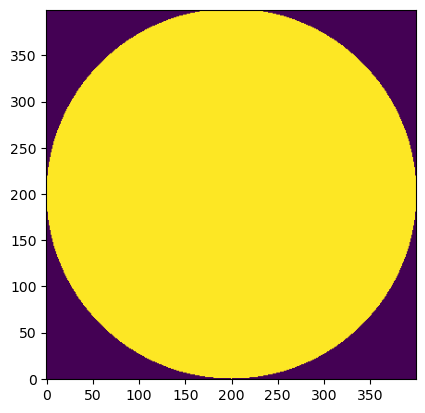
The aperture model is simply an ndarray mask that is True or False for each “sample” of the aperture, depending on whether the light can pass or not. It can also be expressed as an ndarray of floats (0.0 and 1.0).

Circular Aperture with Obscuration

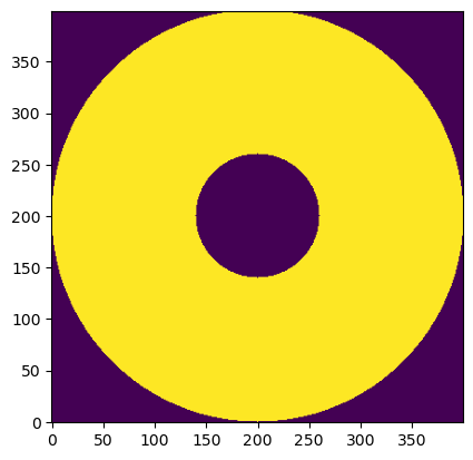
However, this aperture is not very realistic, as Pléiades has a 30% centre obscuration due to the secondary mirror. Now let’s define this aperture.

Also note the use of the extent keyword to map the aperture onto real dimensions.

# 30% obscuration for Pléiades
obscuration_ratio = 0.3

# generate the grid and the aperture
# r in mm and t in radians
aperture = Aperture.circle_aperture_with_obscuration(
    optics.aperture_diameter, obscuration_ratio, samples, with_units=True
)

grid = aperture.grid

# set the aperture in the Optics model
optics.set_aperture_model(aperture)

print(f"aperture diameter: {optics.aperture_diameter}")
print(f"aperture samples: {samples}")
# sample spacing of the aperture definition
# implicitly assumes samples is int and not (int, int)
print(f"aperture sample spacing: {optics.aperture_dx}")

half_ext = optics.aperture_diameter / 2
# visualise the aperture model
# the extent values map the image to real dimensions
# also possible to initialise a RichData object and use plot2d()
plt.imshow(
    aperture.data,
    origin="lower",
    aspect="equal",
)

aperture diameter: 650.0 mm
aperture samples: 400
aperture sample spacing: 1.625 mm

<matplotlib.image.AxesImage at 0x71c81bef16d0>

To make this even more realistic, we will add three spiders.

from prysm.geometry import spider

from opticks.utils.prysm_utils import Grid

# import numpy as np

# print(optics.params.aperture_diameter / 2 * obscuration_ratio * np.cos(240 * u.deg))
# print(optics.params.aperture_diameter / 2 * obscuration_ratio * np.sin(240 * u.deg))

leg_width = 10 * u.mm

try:
    x, y = Grid(samples, optics.aperture_dx).cartesian()
    spider_leg_1 = spider(
        1, leg_width, x, y, rotation=0 * u.deg, center=(-20, 92.5) * u.mm
    )
    spider_leg_2 = spider(
        1, leg_width, x, y, rotation=120 * u.deg, center=(-84.43 + 5, -48.75) * u.mm
    )
    spider_leg_3 = spider(
        1, leg_width, x, y, rotation=240 * u.deg, center=(84.43 - 5, -48.75) * u.mm
    )

    aperture = aperture & spider_leg_1 & spider_leg_2 & spider_leg_3

    plt.imshow(
        aperture.data,
        origin="lower",
        aspect="equal",
    )
except Exception:
    print("Error in prysm, waiting for an update.")

Error in prysm, waiting for an update.

Rectangular Aperture (with prysm)

For the previous examples we have shown the wrapper Aperture in action, but the aperture definitions from prysm can be used for other shapes. There are a lot of interesting examples here.

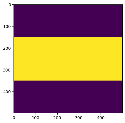
For this example we will define a rectangular aperture with a width of 500 m and aspect ratio of 0.4.

from prysm.geometry import rectangle

# aperture grid definition
sample_size = 500
sample_distance = 1  # in mm

aperture_aspect_ratio = 0.4

# generate aperture grid
x, y = Grid(sample_size, sample_distance).cartesian()

width = int(sample_size / 2)
height = int(width * aperture_aspect_ratio)

# create aperture opening
mask_out = rectangle(width, x, y, height=height, angle=0)

mask = mask_out

# create the Aperture object
rect_aperture = Aperture(mask, grid)

plt.imshow(mask)

<matplotlib.image.AxesImage at 0x71c81bd79090>